This page shows small excerpts of what you can see if you download the
corresponding CDF file. This is "Computable Document Format" of Wolfram.
I made the files with Mathematica. Wolfram no longer provides a plugin, so in
order to see more, you will need to download the CDF file. If you already
have either Mathematica or the free Wolfram CDF Player, then you need
nothing else.
(If you already have Mathematica, you do not need this.)
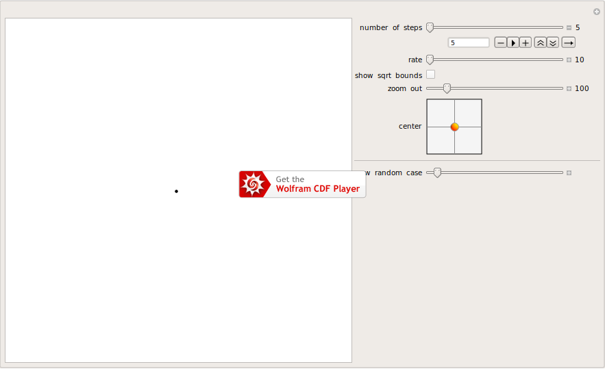
Here we can play with 1-dimensional random walks, thought of as games
where winning and losing has probability 1/2 each, and we keep track
of the number of wins minus the number of losses. You may be surprised at
how infrequently the random walk crosses 0. (You can see one random
instance after another by changing "new random case".) This can be
quantified by the arc sine law.
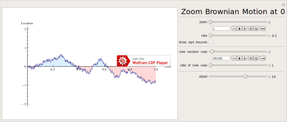
The random walk converges to Brownian motion. You can view Brownian motion
here.
You can zoom Brownian motion at 0 up to a factor of 280.
The vertical scale changes with Brownian scaling, that is, the square
root of the amount of horizontal zooming.
This illustrates the fact that Brownian motion crosses 0 at times
arbitrarily close to 0.
You can choose to display the functions $\pm\sqrt x$ and $\pm2\sqrt x$ for
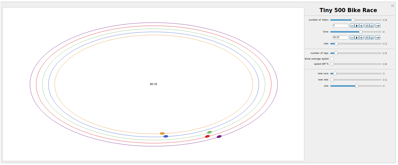
Here is a bicycle race. The race lasts 5 laps (which you can change). Each
rider has a random forward movement during each small increment of time.
All steps are IID and all riders are also IID, unless you choose to make
them have different speeds. The "speed diff" is a percent and will be how
much faster each rider i is than rider i+1 on average. You
can choose to show the average speed of all riders.
The 2-dimensional Brownian motion as Brown viewed it can be seen here:
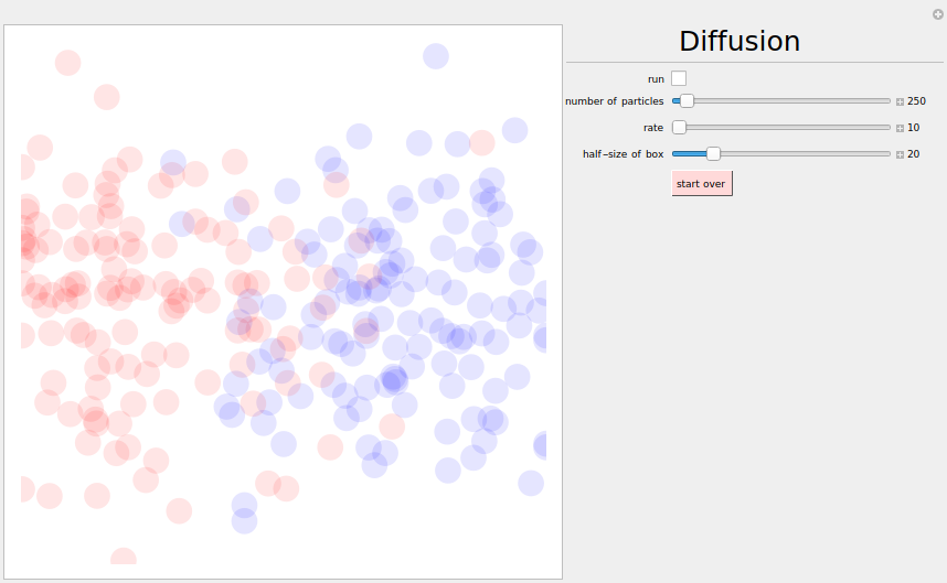
If we have two types of particles, each one performing Brownian motion, we
can see them mix.
You can choose the rate at which the demo updates; for the fastest
possible, make the rate 1000.
'
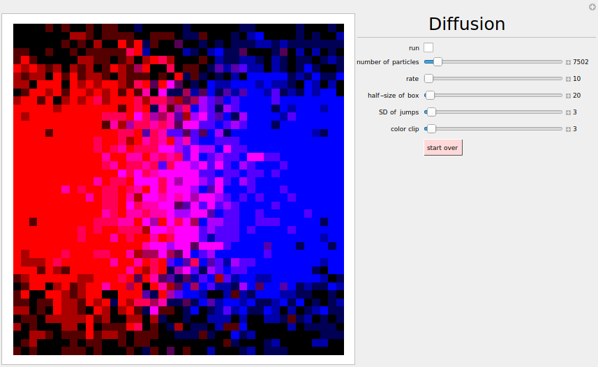
The next demo allows many more particles, each much smaller, but it can be
quite slow with many particles in a large box. You can choose the rate at
which the demo updates; for the fastest possible, make the rate 1000. You
can change "color clip" in order to see varying levels of detail; the value
of "color clip" is the upper limit for the colors, with more particles than
this being truncated at the limit. (More precisely, the number of particles
of each color is divided by this value, and the result is truncated at 1.)
However, it still will not look very smooth as in the real world. The
real world has so many particles (10 grams of water contains about 6 x
1023 molecules of water, Avogadro's number) that it is
essentially the same as continuous. We do not see the discrete nature of
the real world. In fact, Einstein in 1905 gave the first quantitative
explanation of Brownian motion; this gave firm evidence for the existence
of molecules.
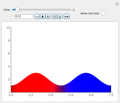
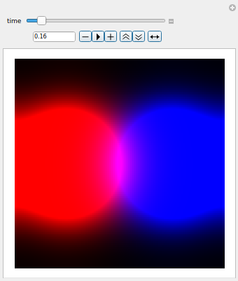
In the following demo, we show the continuous version of diffusion, which
is the expectation of Brownian motion.
The first one is for 1 dimension, while the second is for 2 dimensions.
The 2-dimensional Brownian motion is a limit of 2-dimensional random walks.
In the video, the newest steps are in red, the oldest in blue, and the
intermediate ones in green, so that you can see the time aspect of the
random walk.
Colors are interpolated throughout the walk.
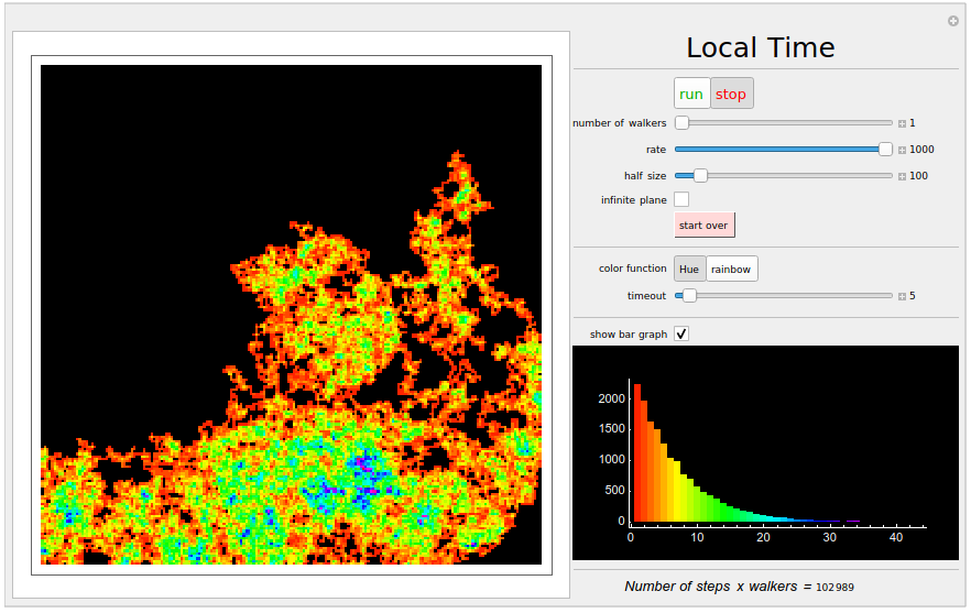
Now we keep track of how many times each site is visited by the random
walker (or by many random walkers), either in the whole plane or restricted to
just a piece of the square lattice with 2n+1 vertices on each side,
where 2n+1 is
"half size". This is known as "local time".
You can choose the rate at which the demo updates; for the fastest
possible, make the rate 1000. You can also display a bar graph showing the
number of sites that have a given local time, i.e., the distribution of the
local time on the sites. The bar graph also gives the color code for the
local time.
If the size is very large, the display can get very slow, and then it
can abort due to a timeout. If that happens, simply increase the timeout.
For some explanation of quantitative phenomena you may observe, see this
paper and this paper.
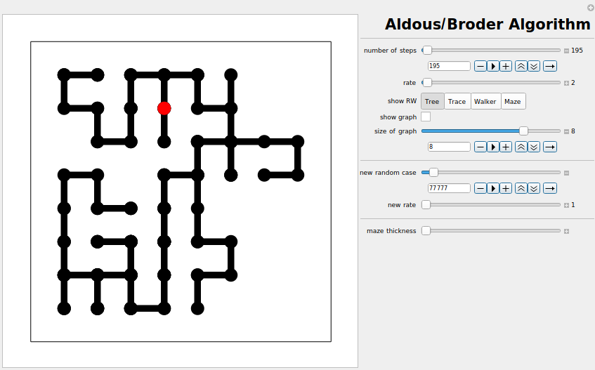
Now we restrict random walk to
just a piece of the square lattice with n vertices on each side,
where n is
"size of graph".
However, we draw an edge only
when the walker arrives at a vertex it has never visited before. The walker will eventually (with probability 1)
visit each of the vertices, and at this point, no new edges will be drawn,
so we might as well stop. What will we see? Take a look!
We got a spanning tree of the graph, i.e.,
a subset of the edges of the graph such that for every
pair of vertices, a and z, of the graph, there is a unique
path of edges in the spanning tree that connects a to z.
Of course, the particular spanning tree that results is random since the
walk is random. What is its distribution?
Amazingly, it is uniformly distributed among all possible spanning trees of
the graph, i.e., all are equally likely!
You can turn this into a maze by increasing the thickness of the edges.
Very interesting phenomena occur when we consider lamps at the locations of
the random walker.
Imagine that a lamplighter must turn on the lamps at all locations, of
which there are infinitely many, one at each integer.
His home is the origin (0), and all lamps are off during the day. However,
as night approaches, he must turn them on. Faced with this impossible
task, he gets drunk and thus walks around at random, switching the state of
the lamp at random as well.
That is, at each time step, he may either walk left 1, walk right 1, or
switch the lamp where he is (on to off or off to on). Each of these 3
choices has probability 1/3 each time, as you can see in the demo below.
A state now consists of the location of the lamplighter as well as the
status of each lamp (on/off). It turns out that these states form a group:
the identity element is where the lamplighter is at 0 and all lamps are
off. Only finitely many lamps can be on; each state can be thought of as a
sequence of (non-random)
instructions to the lamplighter, and group multiplication is
found by composing two such sequences.
How many group elements are within distance
n of the identity? Quite a few: roughly φn, where
φ = (1+ $\sqrt5$)/2 ≅ 1.618
is the golden ratio. (Hint: consider only instructions that never move
left and observe the Fibonacci numbers appear.)
Thus, this lamplighter group has exponential growth. But how fast does the
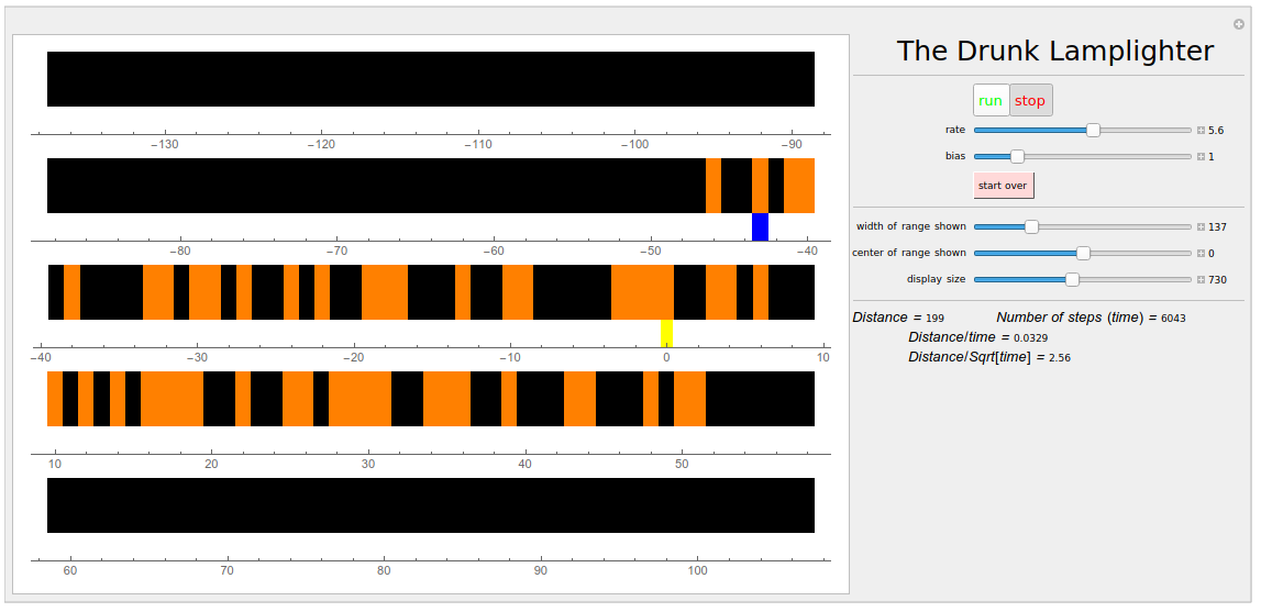
lamplighter move away from the identity?
After n steps, he has usually moved around $\sqrt n$ away from 0
and thus there are roughly $\sqrt n$ lamps on within distance
roughly $\sqrt n$ (as you can see in the demo). This is at
distance only roughly $\sqrt n$ from the identity, so just like
random walk on the integers, the distance increases very slowly, with 0
limiting speed (= distance over time).
As morning approaches, the lamplighter realizes he has a reasonable task of
turning off all lamps and also the effect of the alcohol begins to wear
off.
Thus, while still somewhat drunk, he is more likely to make choices that
decrease his distance to the identity.
In other words, there is some λ > 1 such that each choice that
decreases his distance to the identity has weight λ, while all
other choices have weight 1. This weighting factor λ increases so
that eventually it is infinite and he is no longer drunk. In the demo,
λ is called "bias". You can see that when the bias is large, the
lamplighter quickly manges his task.
What happens when λ is only moderate? It is quite surprising that
when 1 < λ < φ, then actually the lamplighter is worse off:
his speed is positive!
For a proof, see this paper.
There is also a surprise when λ < 1, but I won't spoil it for
you.
What happens if the lamplighter is walking in 2 dimensions? Similar
calculations for the unbiased case (λ = 1) show that again the speed
is 0, but in 3 and more dimensions, the speed is positive. This relies on
Pólya's theorem.
But what about the biased lamplighter in 2 dimensions? No one knows, except
that when λ is smaller than the exponential growth rate, then the
biased random walk is transient, while if λ is larger than the
growth rate, the biased random walk is recurrent (this holds for general
Cayley graphs; see this
paper).
It would be wonderful to see a simulation, but note that a traveling
salesman problem must be solved!
This material is based upon work supported by the National Science
Foundation under Grant No. DMS-1007244.
Any opinions, findings and conclusions or recommendations expressed in this
material are those of the author and do not necessarily reflect the
views of the National Science Foundation (NSF).
 '
'