Here are 1000 steps of simple random walk in the plane.
Use your right mouse button to control playback (control-mouse on a Mac).
What's happening? The walker starts at the origin, (0, 0). Each time step,
the walker moves 1 unit either to the right, left, down, or up, chosen
randomly with probability 1/4 each (independently of past steps).
Pólya's famous theorem says that this random walker is recurrent,
meaning that it will eventually return to the origin with probability 1
and, in fact, will eventually visit every lattice site in the entire
(infinite) plane infinitely many times with probability 1!
You can listen to the random walk here:
The x-coordinate is the left channel and the y-coordinate is
the right channel (best heard on headphones, but be careful the volume is
not too loud).
In musical terms, there are two voices, each starting at A440. At each
time step (1/16th note), one of the voices moves by one tone in the scale
of A major, either up or down, while the other does not move. The choice of
which voice moves--and where--is completely random each time, with all
possibilities being equally likely.
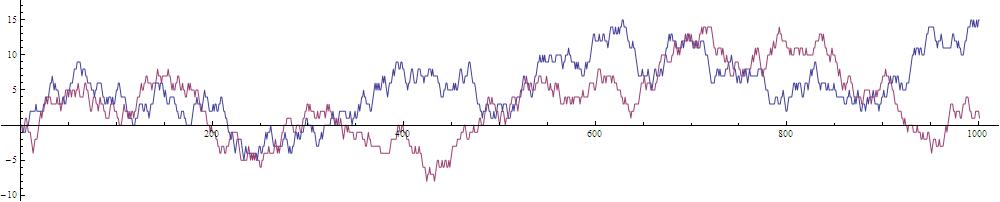
The graph of these two coordinates as a function of time is as follows:
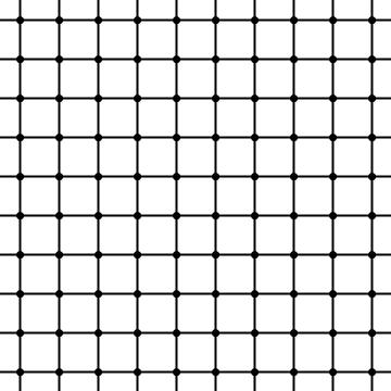
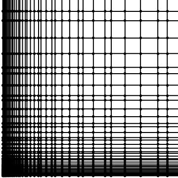
The random walk takes place on a square lattice grid like this (which, by
the way, also exhibits a variation of the scintillating grid illusion):
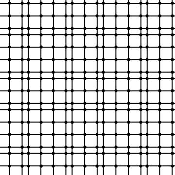
However, since the coordinates were converted to a major scale and the
tones in a scale vary by whole or half tones, it is akin to walking on this
grid:
On the other hand, our hearing is logarithmic, so in terms of pitch
frequencies, it is like walking on this grid:
If we draw every edge the random walker crosses in the above random walk,
we will get an indecipherable mess. However, suppose we draw an edge only
when the walker arrives at a vertex it has never visited before. Let's do
this on a finite (connected) graph, like a 4-by-4 piece of the square
lattice. In this case, the walker will eventually (with probability 1)
visit each of the 16 vertices, and at this point, no new edges will be drawn,
so we might as well stop. What will we see? Take a look:
We got a spanning tree of the graph, i.e.,
a subset of the edges of the graph such that for every
pair of vertices, a and z, of the graph, there is a unique
path of edges in the spanning tree that connects a to z.
Of course, the particular spanning tree that results is random since the
walk is random. What is its distribution?
Amazingly, it is uniformly distributed among all possible spanning trees of
the graph, i.e., all are equally likely!
A uniform random spanning tree (UST)
of a 9-by-9 grid in the plane looks like the
picture on the left here:
There are a lot of spanning trees; in fact, there are
8,326,627,661,691,818,545,121,844,900,397,056 spanning trees of
the 9-by-9 grid.
Surrounding a spanning tree by a curve, one gets a random Peano-like curve
that visits each lattice point exactly once in an 18-by-18 region before
returning to its starting point, as on the right above. In other words,
this curve is a Hamiltonian
cycle in the 18-by-18 grid graph.
(There are other Hamiltonian cycles in the grid graph that don't come by
surrounding spanning trees.)
You can listen to the Peano-like curve, starting in the middle of the
region, here:
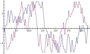
In musical terms, the curve has two voices, each starting at A440. At each
time step (1/16th note), one of the voices moves by one tone in the scale
of A major, either up or down, while the other does not move. The pair of
voices takes each value in an 18-by-18 array of such notes (324 altogether)
exactly once, before returning to its starting point.
The graph of its coordinates is this:
The Peano-like curve has a very interesting scaling limit, i.e., a limiting
random curve in a square if we take finer and finer lattice meshes inside
the square.
This random curve will be "space-filling", i.e., it will visit every point
in the square, even though it never "crosses" itself. It is closely related
to SLE (stochastic Loewner evolution). The SLE processes were
introduced by Oded Schramm and formed a
major part of the work of Schramm, Greg Lawler, and
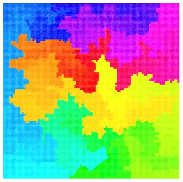
Wendelin Werner that contributed to Werner's earning a Fields Medal. Here
is a picture of a Peano-like curve
from a tree on a 99-by-99 grid, where the hue denotes the
progress along the curve, just like in the movie:
For more information on random spanning trees, go to the
random mazes page or see Chapter 4 in
the book I've written with Yuval
Peres.
The real advantage of sound comes when we do random walk in higher
dimensions, which are harder to represent visually on the screen.
Pólya's theorem says that simple random walk in
any dimension at least 3 is transient, which means that with probability 1,
the walker will return to its starting point only finitely many times and
indeed will never visit any vertex infinitely many times; thus, it wanders
off to infinity.
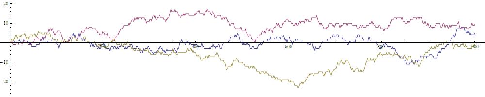
You can listen to 3D random walk here:
The x-coordinate is the left channel, the y-coordinate is
the right channel, and the z-coordinate is in the middle
(best heard on headphones).
The graph of these 3 coordinates as a function of time is as follows:
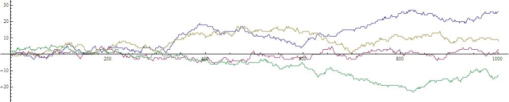
You can listen to 4D random walk here:
The x-coordinate is the left channel, the y-coordinate is
the right channel, the z-coordinate is in the left middle, and
the w-coordinate is in the right middle
(best heard on headphones).
The graph of these 4 coordinates as a function of time is as follows:
For some articles on music theory on other aspects of music that relate to
this kind of representation of notes, see “Geometrical Music
Theory” by Rachel Hall, in Science320 (2008), 328-29,
and the references there.
I created the random walk using Mathematica 7.0.1.0. This is extremely
simple. The following two lines of code create a function rw such
that rw[n,seed] gives a list of vertices in the plane starting
at the origin taking n steps using seed for the random number
generator's seed:
I used the seed 1234. I did not compare to other results and choose the
best-sounding result. I just took what came. I did decide the starting
pitch (A440) and did decide to use the A major scale. I didn't listen to
other choices. I chose to make the random walk steps correspond to 0.2 sec,
just because that seemed right a priori.
For random walk in 3D, I changed the first line above to
Longer random walks would eventually leave the realm of what we can hear.
They would be better restricted to a portion of the grid. Alternatively,
one could take a random walk on a torus and use a Shepard (circular) scale.
I output the notes using Mathematica to write a score using
the free software Lilypond. For the score, I chose 1/16th notes for each
time step, which made the tempo 75 beats per minutes. I chose the time
signature 4/4 since that seemed to fit best walking on a square grid.
Measures were just for convenience in following the piece. For the Peano
curve, I filled out the last measure with the starting note; an alternative
would have been an eternal repeat. Also, 324/16 would have been a natural
time signature.
I also exported the notes to the free software Midge to create midi files,
which are very small. (However, some combinations of browsers and operating
systems can't play midi files, so I also converted to mp3 and ogg.) I
would have liked to have used a pure sine wave, but that doesn't seem to be
supported, so I used the midi patch called square lead, which is fairly
suitable as well.
I would also have liked to fade the random walk pieces to convey the idea
that they go on forever, but fading is not possible in midi.
Instead, I just lowered the volume once.
I drew graphics of the random walk in Mathematica and exported the
result to gif, which makes a fairly small file. Other graphics
were exported to jpg, which is also fairly small.
The movie was made as follows.
The video came from exporting graphics
from Mathematica to avi. They were
combined with the midi sound
in QuickTime Pro and iMovie on a Mac, and exported to wmv,
which seemed to be the best.
Still, the video quality is noticeably degraded.
The Flash (swf) vector-graphics video was made slightly differently.
Graphics were exported as eps frames, which are vector based. These were
converted to ai frames (also vector based) via Adobe Illustrator so that
they could be imported into Adobe Flash. The sound from the previous
video was converted to asnd using Adobe Soundbooth (maybe this wasn't
necessary) and then imported into Flash. The result was exported as swf,
converting the sound to mp3. The QuickTime version of this was produced
simply by exporting as mov. Flash is no longer supported, so it was converted
to webm.
Here is Mathematica code that gives a function t[n]
whose value is the number of spanning trees on an n-by-n grid:
This material is based upon work supported by the National Science
Foundation under Grant No. DMS-1007244.
Any opinions, findings and conclusions or recommendations expressed in this
material are those of the author and do not necessarily reflect the
views of the National Science Foundation (NSF).